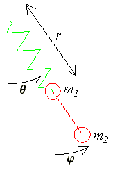
This simulation shows a dangling stick which is a massless rigid stick with a point mass on each end. One end of the stick is attached to a spring, and gravity acts.
You can change parameters in the simulation such as mass, gravity, and damping. You can drag either end of the stick with your mouse to change the starting position. The "reset" button puts the simulation in a motionless equilibrium.
Can you find the bug in this simulation? Play with it for a while and see if you can determine when the bug occurs. Perhaps you can even have a theory for why it occurs. The answer is found below.
The math behind the simulation is shown below. Also available: source code, documentation and how to customize.
The equations of motion are derived by the Lagrangian method. The three independent variables are:
We use subscript 1 for the mass at the spring-stick intersection, and subscript 2 for the mass at the free end of the stick. The cartesian (x, y) position of the point masses is represented by R1, R2. Note that we use bold and overline to indicate a vector quantity.
Other constants are:
First we calculate the kinematics. That is, we find expressions for the positions R1, R2 of the two masses in terms of the independent variables r, θ, φ . Then we differentiate to get the velocities. Note that kinematics is purely an exercise in geometry, there is no information about the forces involved at all.
R1 = {r sin θ, −r cos θ}
R2 = {r sin θ + S sin φ, −r cos θ − S cos φ)}
The two components of the positions correspond to {x, y} respectively. Next differentiate to get the velocities of the masses, v1, v2
R1' = v1 = {r θ' cos θ + r' sin θ, −r' cos θ + r θ' sin θ }
R2' = v2 = {r θ' cos θ + r' sin θ + S φ' cos φ, −r' cos θ + r θ' sin θ + S φ' sin φ}
Next we get separate expressions for the kinetic energy T and potential energy V of the system. The difference of the two is the Lagrangian L = T − V .
Kinetic energy is given by 1⁄2 m v2 . Note that we use the vector dot product to square the velocity vector, v2 = v · v . So we have
T = 1⁄2 m1 v1 · v1 + 1⁄2 m2 v2 · v2
The potential energy is from the spring energy and the gravitational potential of the two point masses.
V = k⁄2 (r − h)2 − m2 g (r cos θ + S cos φ) − m1 g r cos θ
To find the equations of motion, we evaluate the Lagrangian equation once for each of the three independent variables.
$$0 = \frac{d}{dt} \left( \frac{\partial L}{\partial r'} \right) - \frac{\partial L}{\partial r}$$
$$0 = \frac{d}{dt} \left( \frac{\partial L}{\partial \theta'} \right) - \frac{\partial L}{\partial \theta}$$
$$0 = \frac{d}{dt} \left( \frac{\partial L}{\partial \phi'} \right) - \frac{\partial L}{\partial \phi}$$
The three Lagrangian equations can now be solved to find expressions for the second derivatives r'', θ'', φ'' . After using a computer algebra program we find the following equations of motion.
| r'' = | 1 | ( k (2 m1 + m2) (h − r) + 2 m1 (m1 + m2) r θ'2 + 2 g m1 (m1 + m2) cos θ + 2 S m1 m2 φ' 2 cos (θ − φ) − k m2 (h − r) cos(2θ − 2φ) ) | |
| 2 m1 (m1 + m2) |
| θ'' = | 1 | ( k m2 (h − r) sin(2θ − 2φ) − 2 g m1 (m1 + m2) sin θ − 4 m1 (m1 + m2) r' θ' + 2 S m1 m2 φ' 2 sin(θ − φ) ) | |
| 2 m1 (m1 + m2) r |
| φ'' = | k (h − r) sin(θ − φ) |
| S m1 |
This is almost ready for the Runge-Kutta algorithm to numerically solve the equations. All that is needed is to change these 3 second order equations to 6 first order equations by defining separate variables for r', θ', φ' . Let the new variables be respectively vr, vθ, vφ . Then the left-hand side of the above equations of motion become vr', vθ', vφ' and the three additional equations are simply
r' = vr
θ' = vθ
φ' = vφ
There is a problem in the equations of motion when the length of the spring _r goes to zero, because then one of the second derivatives (the one for Qpp ) goes to infinity. If you play with the simulation long enough you will likely see this happen.
Here is my idea for why it blows up: The rate that the angle of the spring changes depends on the torque (twist) applied, which is partially dependent on the length of the spring. When the length goes to zero, the torque goes to infinity.
In the real world, springs never reach zero length. To eliminate this bug, we would need to model the spring with a non-linear force. As the spring compressed to near zero (or to near its smallest possible length) the force would go to infinity.
This web page was first published September 2001.